Correction (Oct 12, 2026): an earlier version of this article stated that Hopiplaka’s book does not cover Goldbach Time. It does — his “Goldbach Time” method uses clock arithmetic (hour + minute of swing pivots). This article’s window-partition method is a different approach in the same family. The comparison is now documented in Section 4.
1. Starting from ICT Principles
Everything in this article derives from three ICT principles you already accept:
Principle 1: Time is half the trade. ICT’s entire methodology rests on when price does things, not just where. The 7AM Model itself is a time thesis: the same setup at the same time every morning. AMD is a time cycle. Killzones are time windows.
Principle 2: The Power of 3 governs market structure. Accumulation, Manipulation, Distribution — three phases. Premium, equilibrium, discount — three zones. Powers of 3 (27, 81, 243, 729) are the fractal signature of how this methodology reads markets.
Principle 3: Price is delivered to specific levels. Order blocks, FVGs, liquidity voids — ICT’s PD arrays form at specific locations. The entire ICT reading of a chart is “which array, at which level.”
Goldbach time levels apply Principle 3 to Principle 1, using Principle 2 as the measuring system. No new doctrine — just the logical extension of what ICT already teaches.
2. The Missing Ruler: Why Time Needs Levels Too
On the price axis, you have surgical tools: “price is at the 50% equilibrium of yesterday’s range.” On the time axis: “we’re in the killzone.” Those are neighborhoods, not levels. A killzone is 90 minutes wide. You can’t time an entry off a neighborhood.
What ICT traders lack is time levels — specific moments within a session where the probability of an event spikes, the temporal equivalent of an order block.
3. The Math: Goldbach Partitions and Powers of 3
Goldbach’s conjecture (1742): every even number greater than 2 is the sum of two primes. The six prime pairs summing to 100:
| Pair | Percentages |
|---|---|
| 3 + 97 | 3%, 97% |
| 11 + 89 | 11%, 89% |
| 17 + 83 | 17%, 83% |
| 29 + 71 | 29%, 71% |
| 41 + 59 | 41%, 59% |
| 47 + 53 | 47%, 53% |
These are the backbone of Goldbach price levels (Hopiplaka, Demystifying ICT, 2023): OB at 11%, FVG at 17%, LV at 29%, BRK at 41%, MB at 47%, EQ at 50%. Powers of 3 (27, 81, 243, 729 minutes) size the time container.
4. The Time Rotation
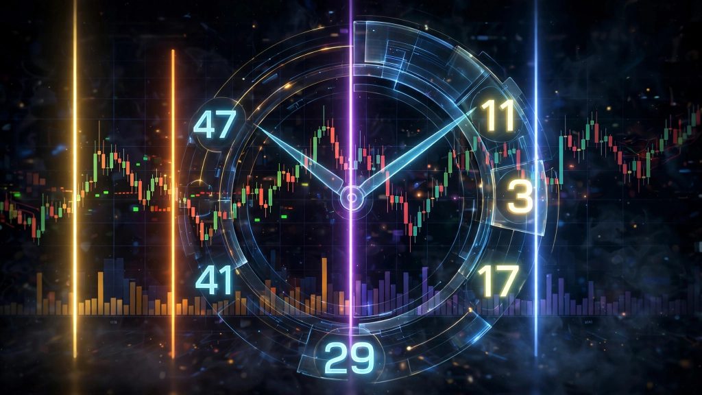
Take the Goldbach price grid and rotate it 90 degrees:
- Price version: 243-point range → horizontal lines at 3/11/17/29/41/47/50%
- Time version: 243-minute window → vertical lines at 3/11/17/29/41/47/50%
The anchor is a time: the 9:30 cash open, midnight, the prior 18:00. If algorithms deliver price to specific levels, they deliver it at specific times too.
A note on what’s original here. Hopiplaka’s Demystifying ICT documents a “Goldbach Time” concept — but it’s a different method: add the hour and minute of a swing pivot’s clock time (e.g., 09:02 → 9+2 = 11), and if the sum is a Goldbach partition number, that swing formed at Goldbach Time. The “Goldbach Time by [Pac]” indicator on TradingView implements Hopi’s clock-arithmetic method and adds a sequence tracker on top. What no one had published before this article is the window-partition method: dividing a PO3 time window into prime-percentage fractions and drawing vertical time levels. Same Goldbach family, different math, different tool.
The Three Goldbach Time Methods Compared
| Hopi (2023) | [Pac] indicator | This article (2026) | |
|---|---|---|---|
| Method | H+M of swing clock time | Hopi’s method + sequence tracker | Prime % of PO3 time window |
| Question answered | “Did this swing form at a Goldbach number?” | “What’s the next time node in the sequence?” | “When in the session do events cluster?” |
| Output | Swing labels (yes/no) | Projected time targets, path table | Vertical time levels on chart |
| Example | Swing at 10:07 → 10+7=17 ✓ | Node hit → next target highlighted | 29% of 243 min → 10:40 line |
Use them together: Hopi’s method confirms swings after they form; the window-partition grid anticipates where in the session to watch. Confirmation plus anticipation is stronger than either alone.
5. PO3 Time Windows
| PO3 | Minutes | Covers | Use |
|---|---|---|---|
| 27 | 27 min | Half a killzone | Scalp sequences, 1m entries |
| 81 | 81 min | One killzone | Micro sessions, AMD single phase |
| 243 | 243 min | ~4 hours | Full morning session |
| 729 | 729 min | ~12 hours | Overnight + cash session |
6. Every Level and Its ICT Meaning
RB Time (3%) — First Probe
The market’s opening test. Early wick, opening-range probe. In AMD terms: accumulation showing its hand.
OB Time (11%) — Institutional Footprint
When real order flow starts printing. Entries here ride the maximum excursion — same logic as entering at an order block in price.
FVG Time (17%) — Imbalance Window
Gaps get created or filled. If price left an early-session FVG, watch for the fill here.
LV Time (29%) — The Launch
The highest-energy moment in the window. When the distribution leg fires: the stop cascade, the trend-leg expansion, the move that defines the session.
BRK Time (41%) — The Flip
Failed morning structure inverts. Support becomes resistance — the breaker in time.
MB Time (47%) — The Return
Pullbacks to origin. The mitigation leg in time.
EQ Time (50%) — Session Equilibrium
Temporal midpoint: pause, balance area, or regime handoff (morning trend → midday chop).
Mirrors (53%–97%)
The grid mirrors around EQ: 53% MB, 59% BRK, 71% LV, 83% FVG, 89% OB, 97% RB. The PM session gets its own structure.
7. Worked Example: 243-Minute Window from the 9:30 Cash Open
| Level | Clock Time | ICT Read |
|---|---|---|
| RB (3%) | 9:37 | Opening range test |
| OB (11%) | 9:57 | Institutional flow arrives |
| FVG (17%) | 10:11 | Gap fill / new imbalance |
| LV (29%) | 10:40 | Distribution leg launches |
| BRK (41%) | 11:10 | Morning levels flip |
| MB (47%) | 11:24 | Pullback to origin |
| EQ (50%) | 11:31 | Mid-session balance |
Note: 10:11 (FVG time) falls inside the 9:00–10:30 killzone; 10:40 (LV time) lands just as it ends. Prime-number math independently rediscovers the killzone boundary.
81-minute micro version from 9:30: RB 9:32 → OB 9:39 → FVG 9:44 → LV 9:53 → BRK 10:03 → MB 10:08 → EQ 10:10. Same structure, compressed for 1-minute sniper entries.
8. How It Maps to AMD
- Accumulation ≈ RB through OB time (3%–11%): positioning, early probes
- Manipulation ≈ FVG through BRK time (17%–41%): stop runs, Judas swing, level flips
- Distribution ≈ LV time outward (29%+): the real move — launched from within manipulation’s extreme, exactly as AMD describes
9. The 81 vs 90 Question
Quarterly Theory uses 90-minute blocks, but 90 isn’t a power of 3. The nearest PO3 window is 81 minutes (3⁴) — 10% shorter, compounding to ~35 minutes of drift by the fourth quarter. Test it: overlay both grids on two weeks of NQ and measure which sits closer to manipulation wicks and distribution launches.
10. Confluence: Time × Price
The highest-probability setup isn’t a time line or price level alone — it’s the cross. PDH tested at LV time (10:40). PDL swept at BRK time (11:10). Two independent systems pointing at the same moment.
Checklist: Where? (horizontal level: PDH/PDL, MNO, NWOG) + When? (time line: LV 29%, BRK 41%, OB 11%) + Which phase? (AMD). Three agree → A++ setup. Two → standard. One → wait.
11. Validate It Yourself: The One-Week Protocol
- Draw the grid (indicator or hand-computed from the tables).
- Each close, mark every manipulation wick (stop-run + reversal ≥ 10 pts) and distribution launch (impulsive leg ≥ 20 pts).
- Record the nearest Goldbach time line and distance in minutes, plus the AMD phase.
- End of week: what % landed within ±5 minutes of a line? Does LV time capture launches?
- Control: generate random times and measure the same. If the grid doesn’t beat random, it’s decoration.
12. The GoldbachTime Indicator
GoldbachTimeV1 for NinjaTrader 8 draws the full grid automatically: vertical dashed lines at every partition + mirrors, any anchor, any PO3 window (27/81/243/729), 5-day history, ICT color coding, each partition toggleable.
Purchase link coming soon.
13. Five Questions Every ICT Trader Will Ask
1. “This is just numerology.”
Nothing in number theory causes order flow — the primes are a ruler, not a mechanism. But the ruler recovers your killzone boundary and nests inside AMD phases. Run the one-week protocol: if it’s numerology, the data will say so.
2. “ICT never taught this.”
ICT taught every ingredient: time matters, AMD is the market’s clock, structures form at levels, PO3 structures everything. This takes ICT’s own principles to their logical conclusion. We’re claiming ICT’s logic, not ICT’s endorsement.
3. “With 13+ lines, price is always near something.”
The lines aren’t evenly spaced — the 17%→29% LV gap is 12% wide, RB sits at 3%. The prime spacing makes specific, falsifiable predictions. Vague grids can’t be tested. This one can — including against a random-time control.
4. “The anchor is arbitrary.”
ICT traders already choose anchors constantly — midnight for the true day, 9:30 for cash, Sunday 18:00 for the week. The anchor is the session you’re trading. Standardize on 9:30/243 for NQ cash.
5. “Institutions would already use it.”
Institutions do use time — VWAP, TWAP, auction imbalances are all time-based execution. Their phase transitions are visible on any chart. The grid names when to look. You don’t need their algorithm; you need their schedule.
14. FAQ
Is Goldbach time part of ICT? No. The window-partition method in this article is PO3Trader’s original contribution (October 2026). It follows ICT’s logic, not ICT’s endorsement. (Hopiplaka documented a different clock-arithmetic Goldbach Time method in Demystifying ICT, 2023 — see Section 4.)
What anchor/window to start with? 9:30 ET anchor, 243-minute window, NQ, intraday chart.
Forex or crypto? The math is instrument-agnostic, but windows assume equity-index sessions. Re-derive anchors for 24h markets.
Daily charts? No — partitions resolve to intraday minutes.
How is this different from Fibonacci time zones? Fib uses the additive sequence; Goldbach uses prime partitions of 100. Different rulers, same bet: time has structure.
Who invented the window-partition time method? PO3Trader — first published October 2026. (Hopiplaka documented the earlier clock-arithmetic method in 2023.)
15. Glossary
- AMD — Accumulation, Manipulation, Distribution: ICT’s three-phase market cycle.
- Anchor — session start time the window is measured from (e.g., 9:30 ET).
- BRK (Breaker) — inverted polarity level; 41% partition.
- Confluence — vertical time line crossing horizontal price level.
- EQ (Equilibrium) — 50%; session midpoint in time.
- FVG (Fair Value Gap) — price inefficiency; 17% partition.
- Goldbach partitions of 100 — (3,97), (11,89), (17,83), (29,71), (41,59), (47,53).
- Killzone — high-volume ICT time window (e.g., NY 8:30–11:00 AM ET).
- LV (Liquidity Void) — origin of violent moves; 29% partition.
- MB (Mitigation Block) — return to origin; 47% partition.
- OB (Order Block) — institutional order zone; 11% partition.
- PD array — premium/discount array: OB, FVG, breaker, MB, LV.
- PO3 — Power of 3; powers of 3 (27/81/243/729).
- RB (Rejection Block) — first range test; 3% partition.
- Time rotation — applying the Goldbach grid to a time window instead of a price range.
GoldbachTimeV1 for NinjaTrader 8 draws the entire grid automatically. Purchase link coming soon.